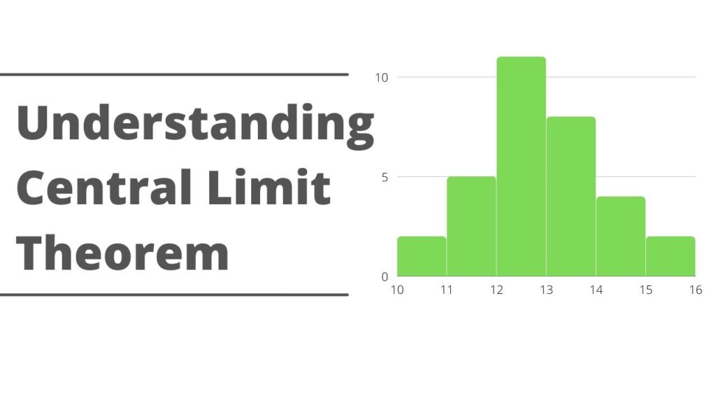
In this article, we will see how to implement Central Limit Theorem with random data. Central Limit Theorem states that the sampling distribution of sample means approaches a normal distribution irrespective of the nature of the population distribution.
The CLT has two properties that we are going to implement here:
1.) Means of Sample Data ~ Mean of the population
2.) Standard deviation(sample) ~ Standard Deviation(population) divided by sqrt(sample_size)
Lets see how can we do this with python.
Import the necessary libraries
import pandas as pd
import numpy as np
import random
import seaborn as sns
Let’s create some random data with the following lines of code.
data = []
for i in range(0,1000):
    n = random.randint(0,100)
    data.append(n)
The above snippet will generate 1000 data points with a random number from 0-100.
Let’s look at the distribution of the data that we have created. It might look something like the below image. It is not normally distributed.
Next, we will create x samples and each sample can contain data of size let’s say 15, so n = 15.
You can change the size of the sample, ideally, you should keep on increasing the sample size for better results.
no_of_samples = 50
n=15
sample_list = []
for i in range(0,no_of_samples):
    samples = random.sample(data,n)
    sample_list.append(samples)
The sample list will look something like this:
Let’s calculate the mean of the sample list we just created. You can do this simply using NumPy.
sample_means = []
for i in range(len(sample_list)):
    sample_mean = np.mean(sample_list[i])
    sample_means.append(sample_mean)
The result will generate 50 means in a list.
Once we have done that, the last step that is left to do is the calculate the mean of all the means that we got above.
This mean of mean should be approximating the actual population mean or the mean of the original data.
mean_of_means = np.mean(sample_means)Since our data is not that large enough we can also calculate the original mean of the population.
original_mean = np.mean(data)When we look at the results below we do see that the values are very much closer to each other. If we increase the sample size it will get better and better.
At the beginning, of the article, we mentioned that the sampling distriution of the means would be a norma distribution irrespective of the population distribution. The below graph proves that the sampling distribution is a normal distribution.
We are using seaborn again to see the histogram plot.
sns.histplot(sample_means, kde=True)The second property to check is the standard deviation of the population that can be calculated using the stdev statistics library in python.
from statistics import stdev
stdev(sample_means)*np.sqrt(n)
stdev(data)
From the below result, we see that the standard deviation of the sample approaches the standard deviation of the population.
I have made a video of this explaining on YouTube as well.
Leave a Reply